Quadrilateral Integration

The integral can be defined as the area between a curve (continuous and differentiable function) and the axis on some given interval.

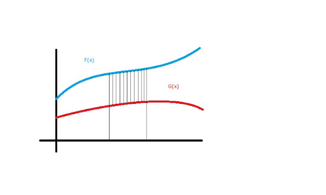
If you want to find the area between two curves that lie on the same interval, it turns out you can subtract one from the other.  So the area in the picture here is _a∫^bF(x) - G(x) dx.
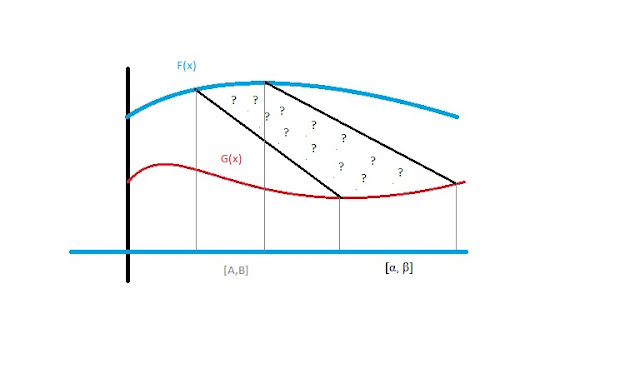
But what if the curves are on different intervals?  How can one determine a function to calculate the area?
A paper I wrote 2/24/2008 explores the area between curves that lie on different intervals.
It does require that for every point in the intervals on which the functions lie, the functions are able to have a line drawn between each other without intersecting.  So each point on curve F essentially must be "in view" of another point on the curve G.  The area between F (on [α,β]) and G (on [a,b]) is:

?AREA? = _α∫^βf(x)dx – _a∫^bg(x)dx + (1/2) * [(α – a)*(f(α) + g(a)) + (b – β)*(f(β) + g(b))]

I have the intervals switched in the picture, but the formula is correct for what I've typed in the line just above... (just put F on (alpha,beta), and G on (a,b) instead of what the picture shows...)

I was going to post the whole paper, proofs and all, but the formatting is weird transferring from MSWord to blog.  So I've taken screen shots of the main points of the 11 page doc.  I've cut out most of the proofs, but leave a comment if you'd like to see them. 

There is a lot of weird notation, but I tried to make it easy to follow.


*** Anything preceded by *** is extra notes outside the paper screen shots...

 *** The proof of this first theorem in mirrors the proof provided at the website: http://www.geometryalgorithms.com/ but they have deleted the original link since this paper was written.

*** Here are the terms I defined to try to explain the quadrilateral integration process.

 *** So the rest of the paper goes on to prove that the limit of this quad sum can be determined... but it does rely on this following theorem.

*** This next theorem is finding the area between a curve on one interval and another interval on the axis, and there is an example to illustrate.



 

*** Next, I find formulas to describe the lines that would form the boundary of the area between F and G.

 *** The picture for example two is a little tough to make out, but I wanted to show the lines C and D intersecting with the X axis. 

*** Theorem 5 is the main point of the paper.  This is the formula shown at the ?AREA? = part...




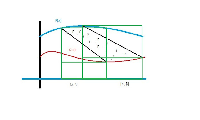
*** Look at this part of that formula...  (1/2) * [(α – a)*(f(α) + g(a)) + (b – β)*(f(β) + g(b))]
*** split it up...                                      (1/2)[(α – a)*(f(α) + g(a))] + (1/2)[(b – β)*(f(β) + g(b))]
*** a litle more...             (1/2)(α – a)*f(α) + 
***                                  (1/2)(α – a)*g(a) +
***                                 (1/2)(b – β)*f(β)  +
***                                 (1/2)(b – β)*g(b)
*** each of these segments is half the area of the green highlighted rectangles in this picture...

***  Using these rectangles, this would be the quick way to determine the area geometrically if the integrals of F and G were known already.  I found it pretty amazing that adding up infinitely many quadrilaterals and taking the limit gives a formula that is essentially identical to the geometrical method.

*** The following corollaries can be derived from the above theorems. 
*** There are a couple examples to illustrate what a few of the corollaries are saying.

 ***  I thought it was interesting that the quadrilateral integration can be done with regards to either axis (X or Y), so long as each F and G have inverses...

 

*** this last corollary is just to point out the connection to an existing discovery...

 *** Well that's the end of the paper....  Pretty much the whole thing now that I've gone back and looked at it, just missing the proofs (comment if you want to see them).

If you have MATLAB, below is the code I wrote to draw examples/compute values
Before you run the code, you have to input the missing values for alpha, beta, a, b; the functions F and G; and then an additional 4 values depending on which functions F and G you choose (in the second FOR loop).


The code will plot the graphs, show the partitions, and then calculate the area based on the partition size chosen.  It is the limit of this value as N reaches infinity that is the actual area between the curves.Quadrilateral Integration (DSB 2008):

alpha = %  the value desired for alpha;
beta = %  the value desired for beta;
a = %  the value desired for a;
b = %  the value desired for b;

     delta = beta - alpha;
     DELTA = b - a;
     x = 0:.1:max(b,beta)+1;

y = %  This is f(x);
y(2,:) = %  This is g(x);

plot(x,y);

n = input('partition size n = ');
     inc = delta/n;

%          this first for loop draws the partition lines%          on the plotted functions.

for i=0:n
     xfi = alpha + i*inc;
     xgi = (DELTA/delta)*(xfi - alpha) + a;
     line([xfi,xgi],[,]);
     i=i+1;
     end

area = 0; %  initialize to zero at the start

%    this second for loop calculates the area.

for i=1:n
xfi = alpha + i*inc;
xfj = alpha + (i-1)*inc;
xgi = (DELTA/delta)*(xfi - alpha) + a;
xgj = (DELTA/delta)*(xfj - alpha) + a;

x1 = xgi;
x2 = xfi;
x3 = xfj;
x4 = xgj;

y1 = % set equal to g(x1) with the actual formula...example, if G(x1) = x1, y1 = x1;
y2 = %  set equal to f(x2)   actual formula... example, if F(x2) = x2+1, y2 = x2+1;  y3 = % set equal to f(x3);
y4 = % set equal to g(x4);

A = (x1*y2-x2*y1)+(x2*y3-x3*y2)+      (x3*y4-x4*y3)+(x4*y1-x1*y4);

area = area + A/2
i=i+1;
end

One, Four, Five!

Here's a way to find out what key a song is in while playing along (and a little music theory)...

Just remember that for any Major key, the first (I), fourth (IV), and fifth (V) notes are always going to be major.  So consider the key of C.

C Scale:     C    D    E     F    G    A    B
Number:     I     ii     iii     IV   V   vi    vii

So we have the One, Four, Five for C major:  C F G

Lets say you're listening to a song, and you can tell it has an A major chord in it.
Using this method, you can quickly find out which key the song is in, and then you'll know which scale to play to fit in.

There are three places this A major chord could fit into the scale, either the first, fourth or fifth position...

1 4 5                   I   ii     iii      IV  V   vi      vii                1 4 5
A _ _   A major (A  Bm  C#m  D  E   F#m  G#m) ==> A D E   is the 1,4,5 for A major
_ A _   E major (E  F#m G#m  A  B  C#m  D#m) ==> E A B  " " " " " " " " " " " E major
_ _ A   D major (D  Em   F#m  G  A  Bm    C#m) ==> D G A " " " " " " " " " " " D major

So from here, you'd want to try to find more chords in the song's progression, and you can narrow down this short list.

Similarly, if all you can find is a minor chord in the song, there will be 4 places in the scale the chord could fit.

Let's say Dm, now we're dealing with 2nd, 3rd, 6th, and 7th positions in the scale (takes a little more time and memorization than the major chord/scale).

2    3 6 7                            I    ii       iii      IV  V   vi      vii                 1  4  5
Dm _ _ _  ==> C major   (C   Dm   Em   F    G   Am   Bm)   ==>    C F G
_ Dm _ _  ==> Bb major  (Bb Cm   Dm   Eb  F   Gm   Am)   ==>   Bb Eb F
_ _ Dm _  ==> F major    (F   Gm   Am   Bb  C   Dm   Em)   ==>  F Bb C
_ _ _ Dm  ==> E major    (E   F#m G#m  A   B   C#m Dm)   ==>    E A B


Practice Tips: 
Try to do the exercise above for another chord other than A major or Dm. 
Try to figure out the chords to a song by ear.

Also,
Play the scale of the key you want.
Then, try to play the chords at each note of the scale. 
Try to mix up which chords are major or minor as you go up the scale, and see how it sounds if you change from the 1,4,5 pattern shown above.  (MAJOR minor minor MAJOR MAJOR minor minor)

Example:
play first the notes: C D E F G A B
then play the chords: C Dm Em F G Am Bm
now see how it sounds to play these chords: C D E F G A B (all major)
or try any other variation from 1,4,5 being major.

The Goldbach Conjecture (an unsolved problem)

The Goldbach conjecture (GBC) has been around in one form or another since the mid-1700s. 
It is easily stated, but has yet to be proven...

The statement:
"Every even number is the sum of two prime numbers"

Is what is known as the "strong Goldbach conjecture".  This was noted in correspondence between two very well known mathematicians of the time, Leonhard Euler and Christian Goldbach.

I am always drawn to study unsolved problems in mathematics because in the past, solutions to such problems have given insight to many other fields, and even require invention of new techniques and models to solve, which advances the science of mathematics even further. 

So here is an introduction to my research on the unsolved Goldbach Conjecture.

From the beginning,
"Every even number is the sum of two prime numbers"

So letting each even number be represented by 2n, we can rewrite this statement as:

2n = p + q    (where p and q are prime numbers less than 2n)

now, it turns out that you can do a little algebraic manipulation to this equation to obtain:

n + n = p + q

which then yields:

n - p = q - n

Now, closely consider this equation...  What this means is that if GBC is true, there is an underlying "symmetry" in the primes.  How?

This arrangement of the equation lets one see that p and q are equidistant from N (which is half of 2n, obviously).  This picture makes it easy to imagine:

So now, what's the big deal?  Why should somebody try rearranging 2n = p + q at all?

IF the GBC is true, this means that for every N, there exist 2 primes, p and q, such that:

1. p < n
2. n < q < 2n    ------>  (see below how this can be n < q < 2n-2 by Bertrand's postulate)
3. neither p or q divide 2n
4. d(p,n) = d(q,n)  (distance function d(x,y)...)

So my goal is to try to force a contradiction in the following manner:

We know that p exists, (any arbitrary prime less than N).
According to Bertrand's postulate,
(if n > 3 is an integer, then there always exists at least one prime p with n < p < 2n − 2)
We know that there must exist some prime q such that n < q < 2n-2
So we can close our bounds on condition 2 above just a little further as indicated above.

It is only left to prove that there exists one prime Q greater than n, less than 2n-2, such that Q-N = N-P, and P does not divide 2n.

IF it can be shown that no such Q can exist, we have contradicted Bertrand's postulate, and therefore GBC must be correct.

But that's the hard part.  I still have yet to find a successful route of attack to force this contradiction. 

Some things to consider if you're going to try to attack it:

1.  Non-prime numbers can be equidistant from prime numbers too...  i.e. 20 = 11+9   but 9 is not prime... How can one guarantee that at least one prime Q (where n < Q < 2n-2) is the same distance from N as a prime less than N?

2.  For each prime P < N, there exists a number N + (N - p) = 2N - P = Q' 
Is there an effective way to check primality of this Q' in each case where P is prime and P < N?  We know that at least one prime number Q must exist in (n, 2n-2), but how do we know which P' < N it is associated with?

From this line of attack I can see two possible ways of proving GBC:
Firstly, by proving the existence of Q for every N and 2N (induction? pigeon-hole principle?).
Or secondly, by assuming Q does not exist and forcing a contradiction to Bertrand's postulate saying that there must be a prime in (n, 2n-2). 

So that's a good introduction so far.  Still no solution as of yet, but I'll keep working on it and see where it goes!